Example Applications

All VisWaterNet scripts should begin with the following steps:

Import the VisWaterNet package.

import viswaternet as vis

Initialize a VisWaterNet model object for the .INP file of the water distribution network. For these examples, we use the CTown network model introduced by Ostfeld (2016).

model = vis.VisWNModel('Networks/CTown.inp')

Alternatively, we can initialize a VisWaterNet model corresponding to a WNTR water network model object.

If you would like to draw the plot into a figure you want to customize yourself (e.g., by drawing into a subplot axis, or by choosing the height and width), import the Matplotlib package and initialize a Matplotlib figure and axis. This is optional; by default, if not provided an empty axis or figure, VisWaterNet will create a figure on behalf of the user.

import matplotlib.pyplot as plt

fig, ax = plt.subplots(figsize=(11,11))
ax.set_frame_on(False)

After we have initialized our VisWaterNet model object, we can proceed to call on different functions offered by the VisWaterNet library to generate a variety of figures. Below, we provide a series of examples to highlight the different VisWaterNet plotting functions and their wide range of inputs.

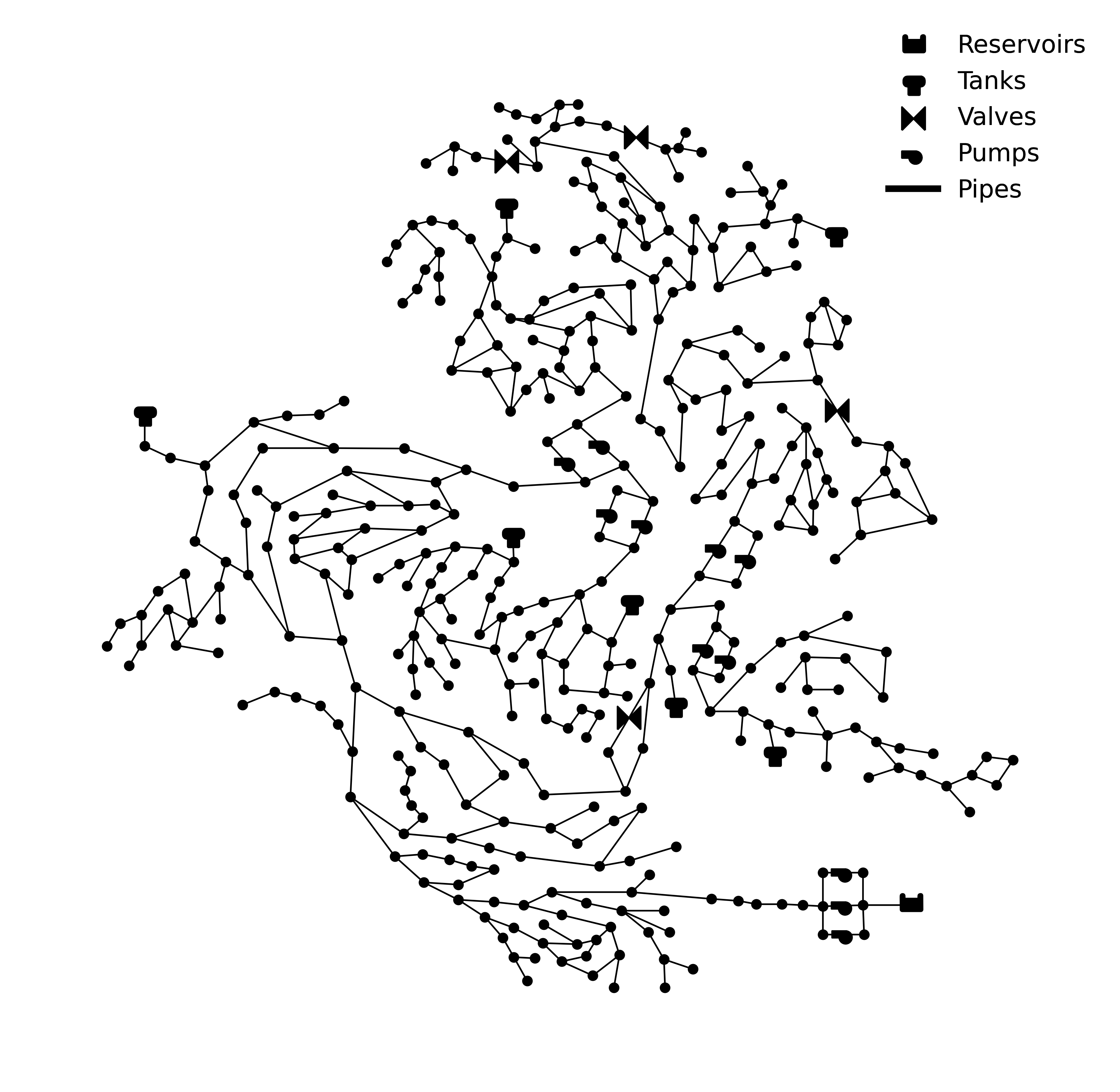
Example 1 - Basic Network Layout Plot

This example demonstrates the basic plotting functionality provided by VisWaterNet. The plot_basic_elements function is used to generate a view of the network layout, depicting the locations of nodes (junctions, tanks, and reservoirs) and links (pipes, pumps, and valves).

model.plot_basic_elements()

Example 2 - Customizing a Basic Network Layout Plot

Here, we customize the basic network plot by changing the location of the legend, color of the tank marker, and pump line style, and draw the figure into axis ax.

model.plot_basic_elements(ax,
                          legend_loc = 'lower left',
                          tank_color = 'g',
                          pump_line_style = ':')

All customization inputs can be found here.

Next, Examples 3 and 4 demonstrate how to visualize data in a continuous manner, i.e., by assigning colors according to a color bar (or gradient scale).

Example 3 - Continuous Node Data Plot for Nodal Pressure

Here, we create a continuous data plot for nodal pressure at hour 10. We increase the size of all nodes to 200 and save the figure as a .PNG file titled ‘example3’ (with resolution 400 dpi) into the figures folder.

model.plot_continuous_nodes(parameter = "pressure", value = 10,
                            min_size = 200, max_size = 200,
                            save_name = 'figures/example3', dpi=400)

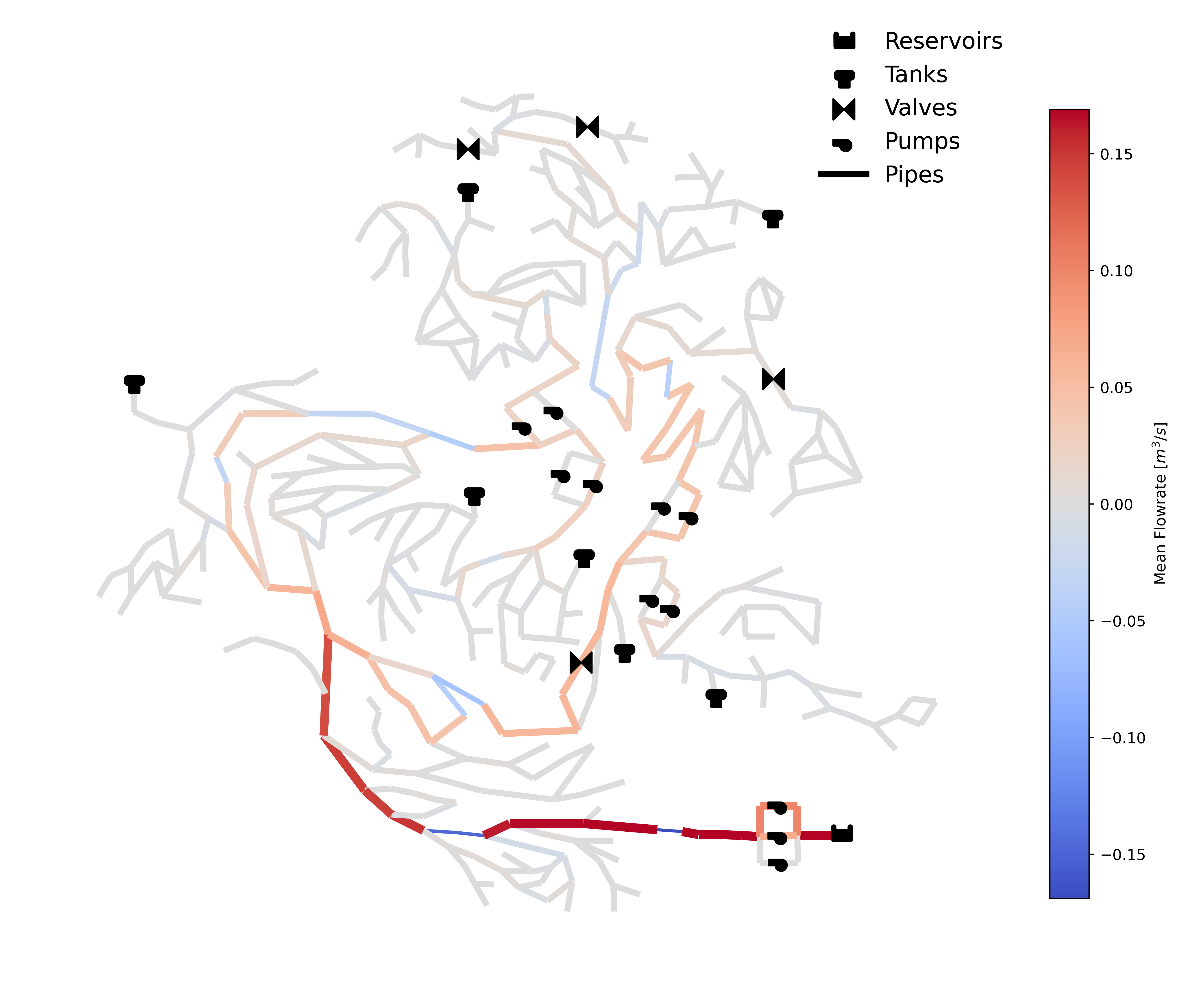
Example 4 - Continuous Data Plot for Link Flow Rate

Here, we create a continuous data plot for mean link flow rate over the simulation duration. We change the color map from the default ‘autumn_r’ to ‘coolwarm’ and vary the width of the links (between min_width and max_width) according to the link flow rate values.

model.plot_continuous_links(parameter = "flowrate", value = 'mean',
                            cmap = 'coolwarm', min_width = 2, max_width = 6)

Next we demonstrate how to visualize data in a discrete manner, i.e., by grouping data into intervals and assigning colors according to each interval shown in a legend.

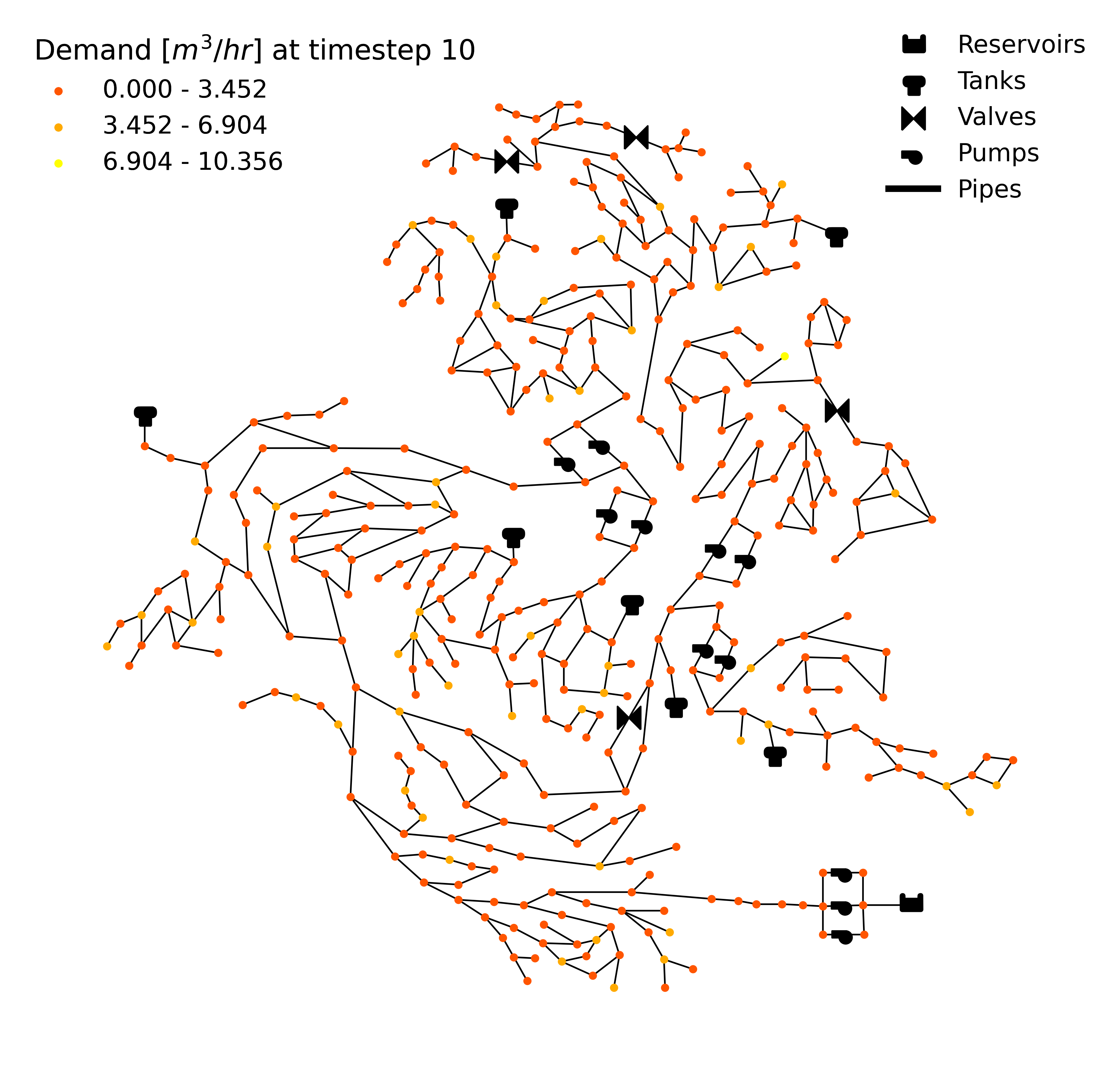
Example 5 - Discrete Data Plot for Nodal Demand

Here, we create a discrete data plot for nodal demand at hour 10. We specify that we want 3 data intervals, change the location of the discrete data legend, and modify the units of the nodal demand from the default flow units (m3/s, following SI convention) to cubic meter per hour (CMH). This is a list of the unit conversion options offered by VisWaterNet.

model.plot_discrete_nodes(parameter = "demand", value = 10,
                          num_intervals = 3,
                          legend_loc_2 = 'upper left', unit = 'CMH')

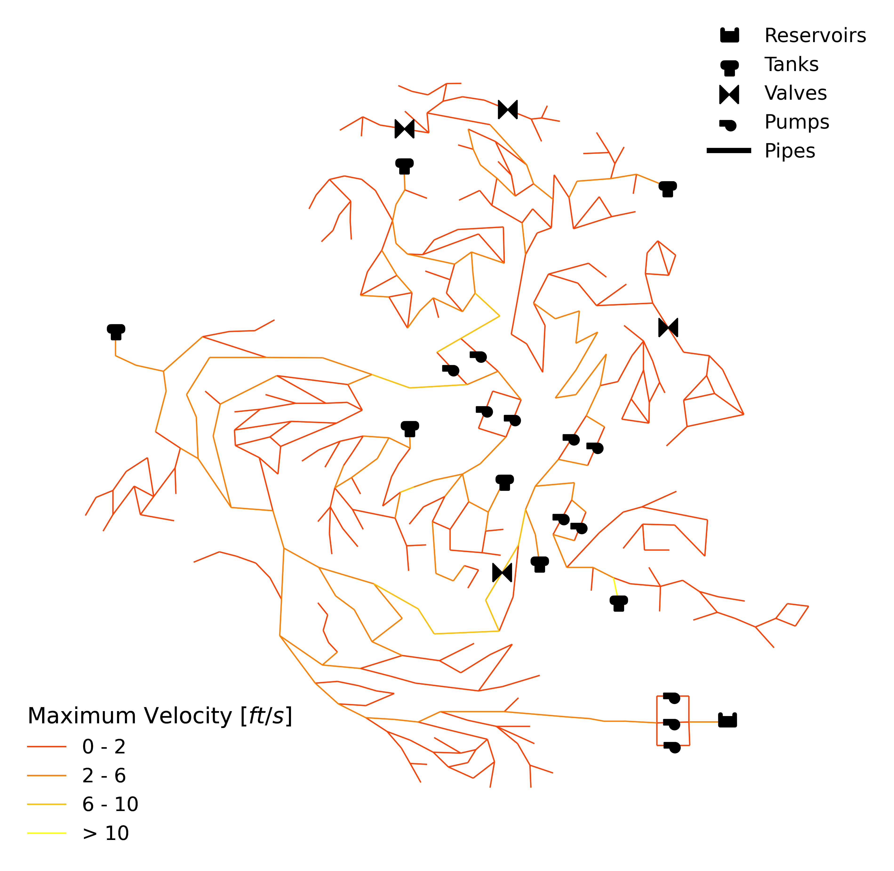
Example 6 - Discrete Data Plot for Link Velocity

Here, we create a discrete data plot for maximum link velocity over the simulation duration. We specify the intervals we would like to see (0-2, 2-6, 6-10). VisWaterNet groups all parameter data into these intervals, and constructs extra intervals (here, <0 or >10) if any data points fall outside of the specified intervals. We customize the legend by specifying that the legend labels should have zero digits after the decimal point (legend_sig_figs=0) and providing a legend title. We also convert the units of velocity to ft/s (from the default SI units of m/s).

model.plot_discrete_links(ax,parameter = "velocity", value = 'max',
                          intervals = [0,2,6,10], legend_sig_figs = 0,
                          legend_loc_2 = 'lower left', unit = 'ft/s')

Next, we demonstrate the different functionalities offered by the plot_unique data function:

visualizing categorical data, i.e., specific properties of nodes or links that belong to a fixed set of categories
importing and visualizing data from an Excel file
visualizing custom data generated within the Python script

Example 7 - Categorical Data Plot for Nodal Demand Pattern

Here, we create a categorical data plot for nodal demand pattern. We modify the color scheme to differentiate clearly between the different demand patterns and modify the legend appearance, location, and labels.

model.plot_unique_data(parameter = "demand_patterns", cmap = 'tab10',
                      legend_loc_2 = 'lower left', legend_title = 'Demand Patterns',
                      legend_title_font_size = 13, font_size = 12,
                      interval_label_list = ['Pattern 1', 'Pattern 2', 'Pattern 3',
                      'Patten 4', 'Pattern 5', 'No Pattern'])

Replacing the parameter value with “diameter” or “roughness” will generate categorical plots for link diameters and link roughness coefficients respectively. Below is an example of a categorical diameter plot.

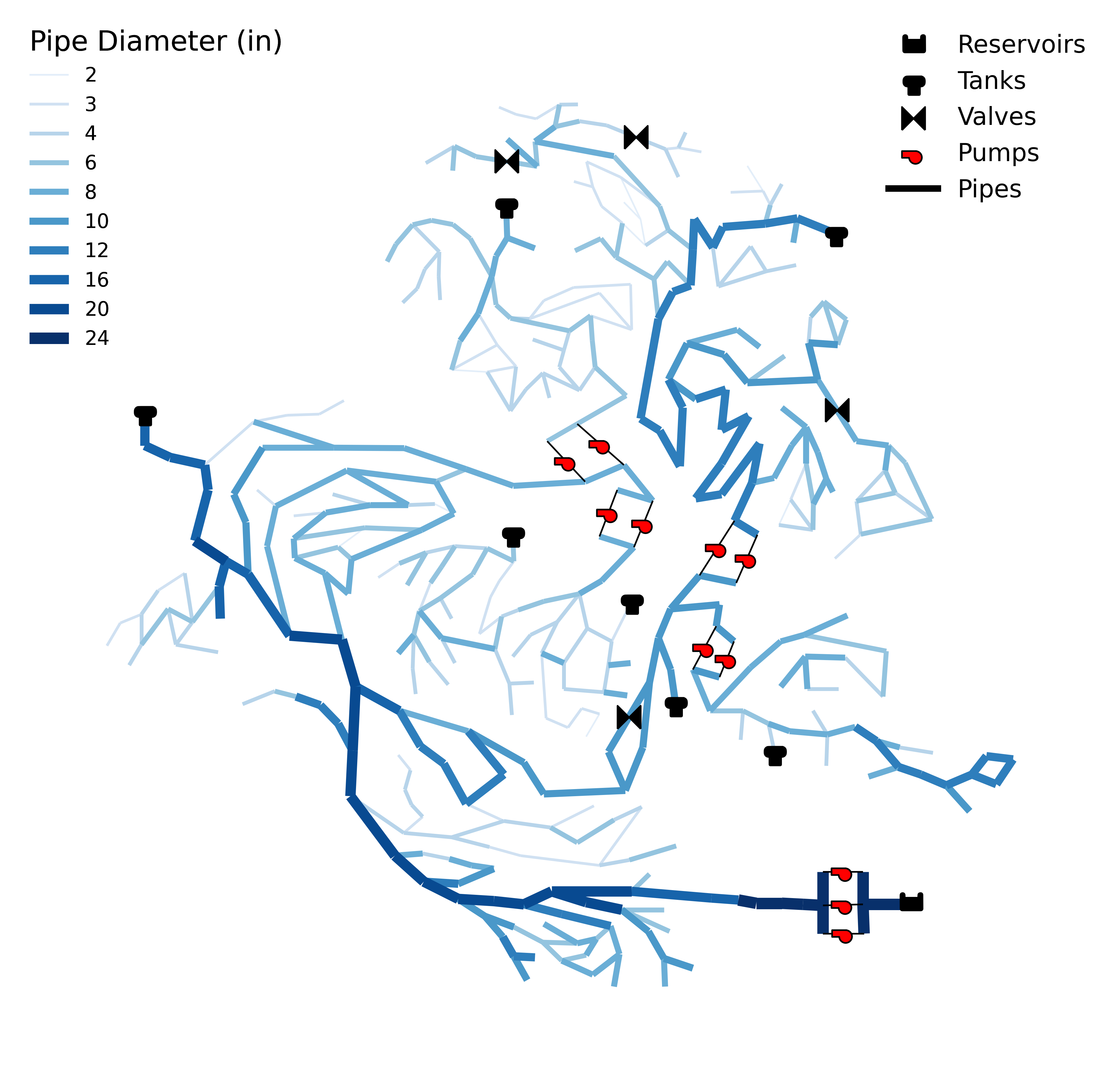
Example 8 - Categorical Data Plot for Link Diameter

Here, we create a categorical data plot for link pipe diameter. In this example we provide several inputs to the function to generate a striking plot highlight different diameter options present in the pipe. First, we import the package NumPy so we can present a linearly spaced list of link widths corresponding to the 10 different unique diameters present in the network to the interval_width_link_list parameter. We then change the color scheme to “Blues” and choose to represent diameters in units of inches (to conform to typical US pipe sizing conventions). Finally, we customize the location and appearance of the legend as well as the appearance of the pumps.

model.plot_unique_data(parameter = "diameter",
                       interval_link_width_list = np.linspace(1,7,10),
                       cmap = 'Blues', unit = 'in',
                       legend_loc_2 = 'upper left',
                       legend_title = 'Pipe Diameter (in)',
                       legend_sig_figs = 0, font_size = 12,
                       pump_color = 'red', pump_width = 2)

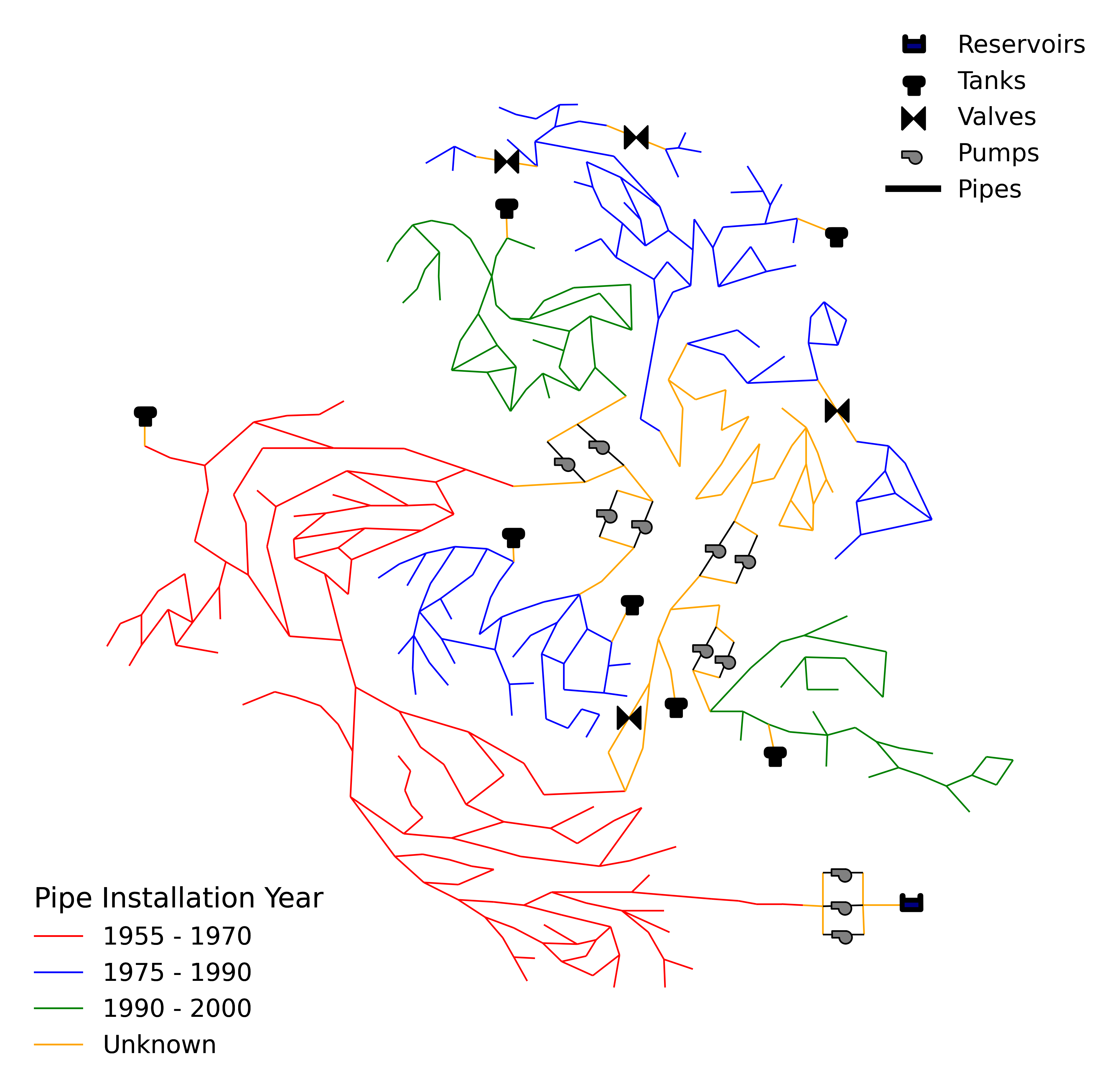
Example 9 - Importing and Plotting Categorical Data from an Excel File

Here, we import data from an excel file named “CTown_pipes_age.xlsx” that has two columns: a column headed “Pipe Name” followed by a list of all pipe names in the CTown network, and a column headed “Year” followed by a list of strings describing the range of years in which the corresponding pipes were installed. We call on the plot_unique data function with parameter = the path name of the Excel file, choose the element we are plotting (parameter_type = ‘node’ or ‘link’), and type of plot we would like to generate: data_type = ‘continuous’ (for a color scale plot of numerical data), ‘discrete’ (for a grouped plot of numerical data) or ‘unique’ (for a plot in which each node/link corresponds to a non-numerical label). The excel_columns input takes in a list of length 2 containing the indices of the columns in the file corresponding to (1) the list of node/link names, and (2) the corresponding data points. Note that the A column of the Excel file is represented by index 0. The dataset in this example contains four unique categories of data, and we choose the colors corresponding to each interval instead of interpolating from a colormap.

model.plot_unique_data(parameter='Excel/CTown_pipe_ages.xlsx',
                       parameter_type='link', data_type='unique',
                       excel_columns=[0,1],
                       color_list = ["red", "blue", "green","orange"],
                       legend_loc_2 = 'lower left', , tank_color = 'k',
                       pump_color = 'gray', reservoir_color = 'navy',
                       legend_title = 'Pipe Installation Year')

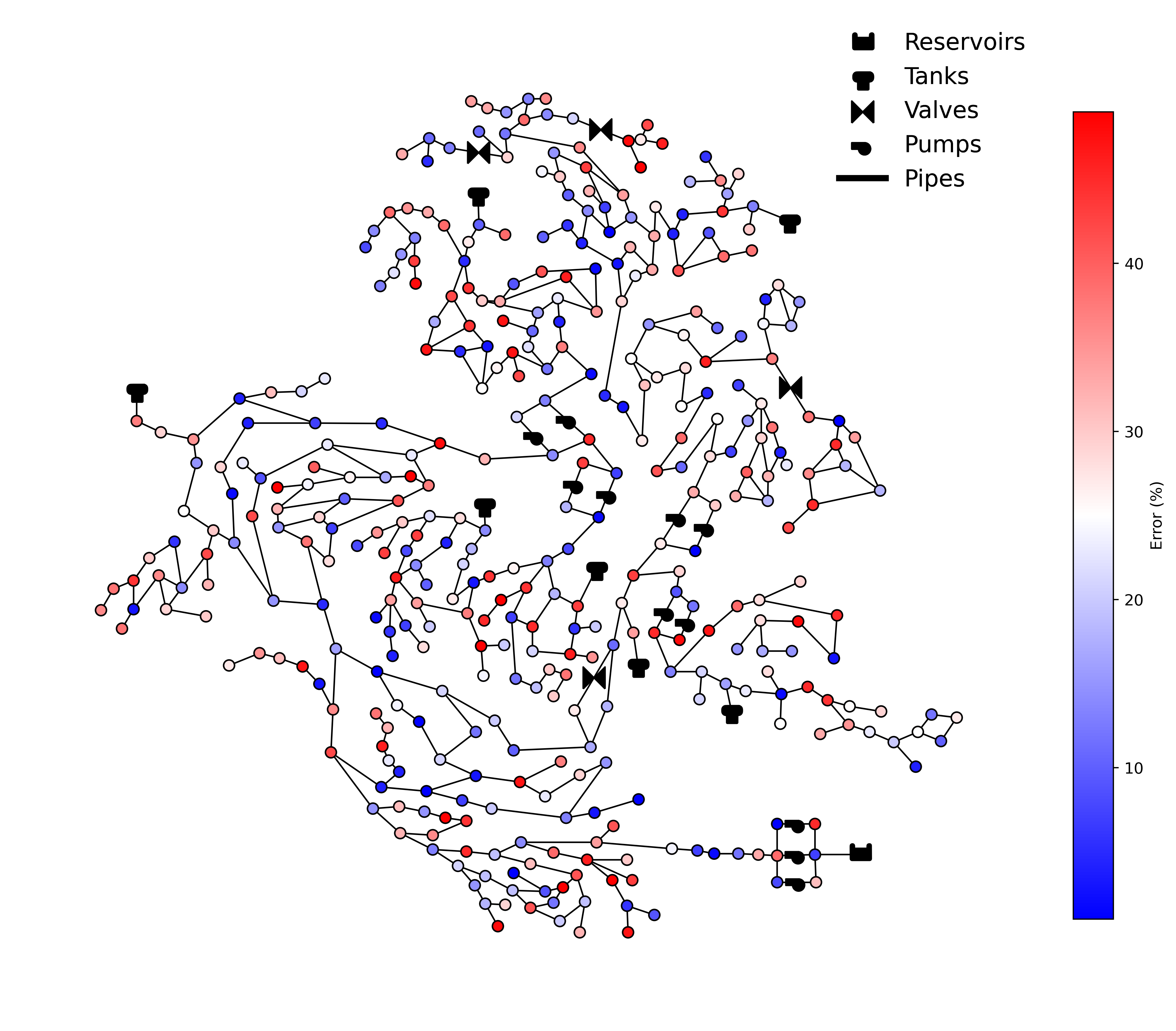
Example 10 - Plotting Custom Data Generated Within a Python Script

Here, we demonstrate how lists of data corresponding to nodes or links can be easily visualized using VisWaterNet. This functionality is useful for plotting results of analyses performed on the water network within Python scripts. We call on the plot_unique data function with parameter = ‘custom_data’, choose the element we are plotting (parameter_type = ‘node’ or ‘link’), and type of plot we would like to generate: data_type = ‘continuous’, ‘discrete’ or ‘unique’. element_list is a list of the nodes or links in the model, and data_list is the list of corresponding data points we would like to plot. In this example, we generate a random set of values in data_list to serve as our data points, and plot them in a continuous manner.

import random

element_list = wn.junction_name_list
data_list = [random.randrange(1, 50, 1) for i in range(wn.num_junctions)]

model.plot_unique_data(parameter = 'custom_data', node_size = 200,
                       parameter_type = 'node', data_type = 'continuous',
                       line_widths = 1, edge_colors = "k",
                       custom_data_values = [element_list, data_list],
                       color_bar_title = "Error (%)", cmap = "bwr")

Example 11 - Creating GIFs

VisWaterNet offers a function that generates time-varying representations of network properties. Here, we demonstrate how to use the animate_plot function to generate a .GIF file showing link flow rate change in a continuous manner over the simulation duration. To generate an animation, we have to provide the following inputs:

ax: a Matplotlib axis that can hold the frames
function: the specific function we want to invoke on model for each frame, e.g., model.plot_discrete_nodes
data_type: the type of plot we wish to generate (‘continuous’, ‘discrete’, or ‘unique’)
parameter_type: the elements we are plotting (‘node’ or ‘link’)
parameter: the node/link parameter data we intend to plot (e.g. ‘flowrate’, ‘pressure’, etc.)
first_timestep: the starting time step of the animation (optional)
last_timestep: the ending time step of the animation (optional)
unit: the time step units shown on the plot (‘min’, ‘hr’, ‘day’, default ‘s’) (optional)
fps: the animation framerate as an integer value (optional)

Additional parameters can be provided to customize the frames as shown in previous examples.

model.animate_plot(ax, function = model.plot_continuous_links ,
                   data_type = 'continuous', parameter_type = 'link',
                   parameter = 'flowrate',
                   first_timestep = 0, last_timestep = 40,
                   unit = 'hr',  fps = 7,
                   max_width = 5, min_width = 5, legend = False,
                   color_bar_title = 'Flowrate [m3/s]',
                   pump_color = 'green', cmap = 'coolwarm')

More examples can be found in the Examples folder. The full range of inputs for each plotting function can be found in this section.